A smart and talented friend, who’s a fellow data scientist by profession, came across a probability puzzle that’s supposedly given in some job interviews for data science roles. The problem asks the following:
Assume the distribution of children per family is such that the probability of having 0 children is 0.30, 1 child is 0.25, 2 children is 0.20, 3 children is 0.15, 4 children is 0.10, and 5 or more children is 0. Consider a random girl in the population of children. What is the probability that she has a sister?
Checking her work, my friend disagreed with the answers she found online, and wanted to know how I’d solve the problem. Since my solution seems to be different than others I’ve found so far, I thought I’d share it with the whole Internet, which will certainly tell me whether I’m wrong.
Simulating the problem
I’ll start with a simulation—I’m a bit more confident in my programming than my probability theory (I’ve been doing it longer), and it makes some of the tricky parts of the problem explicit.
First, we’ll simulate a random sample of families, since the problem gives us probabilities in terms of children per family. After generating a pool of random family sizes, we can use the binomial distribution to generate a random number of girls for each family (naively assuming that the probability of a child being a girl is 0.5).
set.seed(232636039)
num_families <- 100000

family_size <- seq(0, 5)
p_family_size <- c(0.3, 0.25, 0.20, 0.15, 0.1, 0.0)

girls_per_family <- sample(family_size, num_families, replace = TRUE,
                           prob = p_family_size) |>
  (\(n) rbinom(num_families, size = n, prob = 0.5))()
If a family has more than two girls, these girls have sisters. The probability that a randomly selected girl has a sister is approximated by the number of girls with sisters divided by the total number of girls in our simulation.
# If there is more than one girl in a family, these girls have sisters
girls_with_sisters <- sum(girls_per_family[girls_per_family > 1])
girls_total <- sum(girls_per_family)

(p_est <- girls_with_sisters / girls_total)
## [1] 0.5878486
The code above estimates that the probability that a girl (sampled at random from the population of children) has a sister is approximately 0.59.
Plotting the simulation
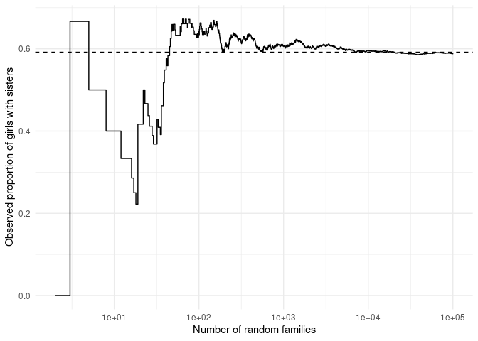
Just for fun, let’s plot the estimate as it develops over the number of simulated families. This also helps us get a sense of how trustworthy the estimate is—has it converged to a stable value, or is it still swinging around? For this, I’ll finally use parts of the Tidyverse.
suppressPackageStartupMessages(library(dplyr))
suppressPackageStartupMessages(library(ggplot2))
sister_dat <- tibble(girls_per_family) |>
  mutate(families = seq(n()),
         has_sister = girls_per_family > 1,
         total_girls = cumsum(girls_per_family),
         girls_with_sisters = cumsum(girls_per_family * has_sister),
         p_est = girls_with_sisters / total_girls)
sister_dat |>
  # We'll skip any beginning rows that were generated before we sampled girls,
  # since 0/0 is undefined.
  filter(total_girls > 0) |>
  ggplot(aes(families, p_est)) +
  geom_step() +
  geom_hline(yintercept = 71/120, linetype = "dashed") +
  scale_x_log10() +
  theme_minimal() +
  labs(x = "Number of random families", y = "Observed proportion of girls with sisters")

Analytic solution
If you’re wondering how I chose a value for the dashed line, here’s an analytic solution to the puzzle.
We’ll let S represent the event that a girl has a sister, Fₙ represent the event that a family has n children, and Cₙ represent the event that a girl comes from a family of n children (i.e., the girl has n - 1 siblings). By the law of total probability:
$$ \mathbb{P}(S) = \sum_{n} \mathbb{P}(S|C_n) \mathbb{P}(C_n) $$
The conditional probability that a girl from a family with n children has a sister is the compliment of the probability that all of her siblings are brothers. Therefore:
$$ \mathbb{P}(S|C_n) = 1 - \frac{1}{2^{n-1}} $$
For the next component, it’s important to call out the fact that the problem text gives us P(Fₙ) (the probability that a family has n children), which is not the same as P(Cₙ) (the probability that a child comes from a family with n children). I suspect that this trips some people up, and explains some of the answers that are different than mine.
To illustrate the difference, let’s imagine that the probabilities were constructed from a population of 100 families. Twenty five of these families have one child, while only ten have four children. However, this arrangement results in 25 children with no siblings, while 40 children would have 3 each. In other words, a randomly selected family is more likely to have one child than four children, but a randomly selected child is more likely to come from a family with four children than a family with one child. Formalizing this reasoning a bit, we find:
$$ \mathbb{P}(C_n) = \frac{n \mathbb{P}(F_n)}{\sum_{m} m \mathbb{P}(F_m)} $$
With our terms defined, we’ll use R once more to calculate P(S):
n <- family_size
fn <- p_family_size
s_given_cn <- 1 - 1/(2^(n-1))
cn <- n * fn / sum(n * fn)
(s <- sum(s_given_cn * cn))
## [1] 0.5916667
This value is equal to 71/120, and is quite close to what we found
through simulation—but only reliably so after generating around 10,000
families.
Concluding note
I’m ambivalent about the practice of asking job applicants to solve probability puzzles during interviews, but it’s true that sometimes our intuitions can lead us astray (e.g, confusing P(Fₙ) and P(Cₙ)), and this does come up in real-life data analyses. When I find myself dealing with such situations, I’m flexible in the approach I take: sometimes I try to find an exact solution using probability theory first, but often I program a quick simulation instead. Most of the time, I wind up doing both, because these approaches complement one another: simulations are great because they force you to be explicit about the assumptions that you’re making about the problem, while analytic solutions give exact answers and are insensitive to randomness.