Introduction
In a previous post, I presented an analysis of data by Horne, Powell, Hummel & Holyoak, (2015) that investigated changes in attitudes toward childhood vaccinations. The previous analysis used Bayesian estimation to show a credible increase in pro-vaccination attitudes following a “disease risk” intervention, but not an “autism correction” intervention.
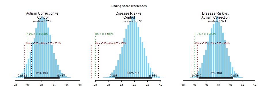
Some of my friends offered insightful comments, and one pointed out what appeared to be a failure of random assignment. Participants in the “disease risk” group happened to have lower scores on the pre-intervention survey and therefore had more room for improvement. This is a fair criticism, but a subsequent analysis showed that post-intervention scores were also higher for the “disease risk” group, which addresses this issue.

Bootstrapping
Interpreting differences in parameter values isn’t always straightforward, so I thought it’d be worthwhile to try a different approach. Instead of fitting a generative model to the sample, we can use bootstrapping to estimate the unobserved population parameters. Bootstrapping is conceptually simple; I feel it would have much wider adoption today had computers been around in the early days of statistics.
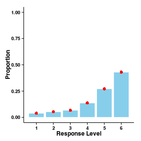
Here is code that uses bootstrapping to estimate the probability of each response on the pre-intervention survey (irrespective of survey question or intervention group assignment). The sample mean is already an unbiased estimator of the population mean, so bootstrapping isn’t necessary in this first example. However, this provides a simple illustration of how the technique works: sample observations with replacement from the data, calculate a statistic on this new data, and repeat. The mean of the observed statistic values provides an estimate of the population statistic, and the distribution of statistic values provides a measure of certainty.
numBootstraps <- 1e5  # Should be a big number
numObservations <- nrow(questionnaireData)
uniqueResponses <- sort(unique(questionnaireData$pretest_response))
interventionLevels <- levels(questionnaireData$intervention)

# The observed proportion of responses at each level
pretestResponseProbs <- as.numeric(table(questionnaireData$pretest_response)) /
  numObservations
# Bootstrap to find the probability that each response will be given to pre-test
# questions.
pretestData <- array(data = 0,
                     dim = c(numBootstraps,
                             length(uniqueResponses)),
                     dimnames = list(NULL,
                                     paste(uniqueResponses)))

# Run the bootstrap
for (ii in seq_len(numBootstraps)) {
  bootSamples <- sample(questionnaireData$pretest_response,
                        numObservations,
                        replace = TRUE)
  bootSamplesTabulated <- table(bootSamples)
  pretestData[ii, names(bootSamplesTabulated)] <- bootSamplesTabulated
}

# Convert the counts to probabilities
pretestData <- pretestData / numObservations

As expected, the bootstrap estimates for the proportion of responses at each level almost exactly match the observed data. There are supposed to be error-bars around the points, which show the bootstrap estimates, but they’re obscured by the points themselves.
Changes in vaccination attitudes
Due to chance alone, the three groups of participants (the control group, the
“autism correction” group, and the “disease risk” group) showed different
patterns of responses to the pre-intervention survey. To mitigate this issue,
the code below estimates the transition probabilities from each response on the
pre-intervention survey to each response on the post-intervention survey, and
does so separately for the groups. These are conditional probabilities, e.g.,
P(post-intervention rating = 4 | pre-intervention rating = 3).
The conditional probabilities are then combined with the observed
pre-intervention response probabilities to calculate the joint probability of
each response transition (e.g., P(post-intervention rating = 4 ∩ pre-intervention rating = 3)). Importantly, since the prior is agnostic to
subjects’ group assignment, these joint probability estimates are less-affected
by biases that would follow from a failure of random assignment.
# preintervention responses x intervention groups x bootstraps x postintervention responses
posttestData <- array(data = 0,
                      dim = c(length(uniqueResponses),
                              length(interventionLevels),
                              numBootstraps,
                              length(uniqueResponses)),
                      dimnames = list(paste(uniqueResponses),
                                      interventionLevels,
                                      NULL,
                                      paste(uniqueResponses)))

for (pretestResponse in seq_along(uniqueResponses)) {
  for (interventionLevel in seq_along(interventionLevels)) {
    # Get the subset of data for each combination of intervention and
    # pre-intervention response level.
    questionnaireDataSubset <- filter(questionnaireData,
                                      intervention == interventionLevels[interventionLevel],
                                      pretest_response == pretestResponse)
    numObservationsSubset <- nrow(questionnaireDataSubset)

    # Run the bootstrap
    for (ii in seq_len(numBootstraps)) {
      bootSamples <- sample(questionnaireDataSubset$posttest_response,
                            numObservationsSubset,
                            replace = TRUE)
      bootSamplesTabulated <- table(bootSamples)
      posttestData[pretestResponse,
                   interventionLevel,
                   ii,
                   names(bootSamplesTabulated)] <- bootSamplesTabulated
    }

    # Convert the counts to probabilities
    posttestData[pretestResponse, interventionLevel, , ] <-
      posttestData[pretestResponse, interventionLevel, , ] / numObservationsSubset
  }

  # Convert the conditional probabilities to joint probabilities using the
  # observed priors on each pretest response.
  posttestData[pretestResponse, , , ] <- posttestData[pretestResponse, , , ] *
    pretestResponseProbs[pretestResponse]
}
With the transition probabilities sampled, it’s possible to test the hypothesis: “participants are more likely to shift toward a more pro-vaccine attitude following a ‘disease risk’ intervention than participants in control and ‘autism correction’ groups.” We’ll use the previously-run bootstrap samples to compute the each group’s probability of increasing scores.
posttestIncrease <- array(data = 0,
                          dim = c(numBootstraps,
                                  length(interventionLevels)),
                          dimnames = list(NULL,
                                          interventionLevels))

for (interventionLevel in seq_along(interventionLevels)) {
  for (pretestResponse in seq_along(uniqueResponses)) {
    for (posttestResponse in seq_along(uniqueResponses)) {
      if (posttestResponse > pretestResponse) {
        posttestIncrease[, interventionLevel] <- posttestIncrease[, interventionLevel] +
          posttestData[pretestResponse, interventionLevel, , posttestResponse]
      }
    }
  }
}
This estimates the probability that post-intervention responses from the “disease risk” group have a greater probability of being higher than their pre-intervention counterparts than responses from the “autism correction” group.
sum(posttestIncrease[, which(interventionLevels == "Disease Risk")] >
      posttestIncrease[, which(interventionLevels == "Autism Correction")]) /
  nrow(posttestIncrease)
## [1] 0.99992
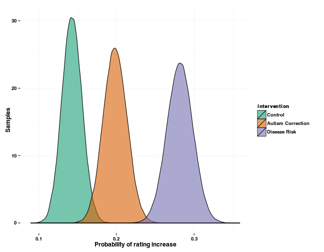
Below is a visualization of the bootstrap distributions. This illustrates the certainty of the estimates of the probability that participants would express stronger pro-vaccination attitudes after the interventions.

Conclusion
Bootstrapping shows that a “disease risk” intervention has a stronger effect than others in shifting participants’ pro-vaccination attitudes. This analysis collapses across the five survey questions used by Horne and colleagues, but it would be straightforward to extend this code to estimate attitude change probabilities separately for each question.
Although there are benefits to analyzing data with nonparametric methods, the biggest shortcoming of the approach I’ve used here is that it can not estimate the size of the attitude changes. Instead, it estimates that probability of pro-vaccination attitude changes occurring, and the difference in these probabilities between the groups. This is a great example of why it’s important to keep your question in mind while analyzing data.